Problem With Many Variables
This example solves a graph problem with too many variables to fit onto the QPU.
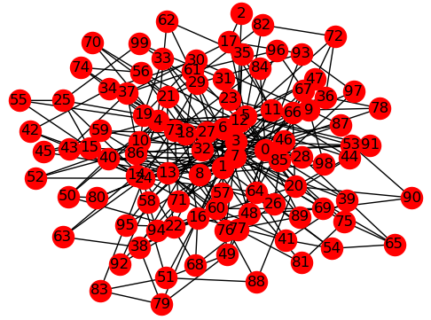
Problem Graph with Many Variables.
The purpose of this example is to illustrate a hybrid solution—the combining of classical and quantum resources—to a problem that cannot be mapped in its entirety to the D-Wave system due to the number of its variables. Hard optimization problems might have many variables; for example, scheduling or allocation of resources. In such cases, quantum resources are used as an accelerator much as GPUs are for graphics.
Note
Currently Ocean tools are not optimized for very large problems. For fully connected graphs, the number of edges grows very quickly with increased nodes, degrading performance. The current example uses 100 nodes but with a degree of three (each node connects to three other nodes). You can increase the number of nodes substantially as long as you keep the graph sparse.
Example Requirements
To run the code in this example, the following is required.
- The requisite information for problem submission through SAPI, as described in Using a D-Wave System.
- Ocean tools dwave-system, dimod, and dwave-hybrid.
If you installed dwave-ocean-sdk
and ran dwave config create, your installation should meet these requirements.
Solution Steps
Section Solving Problems on a D-Wave System describes the process of solving problems on the quantum computer in two steps: (1) Formulate the problem as a binary quadratic model (BQM) and (2) Solve the BQM with a D-wave system or classical sampler. This example uses dwave-hybrid to combine a tabu search on a CPU with the submission of parts of the (large) problem to the D-Wave system.
Formulate the Problem
This example uses a synthetic problem for illustrative purposes: a NetworkX generated graph, NetworkX barabasi_albert_graph(), with random +1 or -1 couplings assigned to its edges.
# Represent the graph problem as a binary quadratic model
import dimod
import networkx as nx
import random

graph = nx.barabasi_albert_graph(100, 3, seed=1)  # Build a quasi-random graph
# Set node and edge values for the problem
h = {v: 0.0 for v in graph.nodes}
J = {edge: random.choice([-1, 1]) for edge in graph.edges}
bqm = dimod.BQM(h, J, offset=0, vartype=dimod.SPIN)
Create a Hybrid Workflow
The following simple workflow uses a RacingBranches class to iterate two
Branch classes in parallel: a tabu search, InterruptableTabuSampler,
which is interrupted to potentially incorporate samples from subproblems (subsets of the problem
variables and structure) by EnergyImpactDecomposer | QPUSubproblemAutoEmbeddingSampler | SplatComposer, which decomposes the
problem by selecting variables with the greatest energy impact, submits these to
the D-Wave system, and merges the subproblem’s samples into the latest problem samples.
In this case, subproblems contain 30 variables in a rolling window that can cover up
to 75 percent of the problem’s variables.
# Set a workflow of tabu search in parallel to submissions to a D-Wave system
import hybrid
workflow = hybrid.Loop(
   hybrid.RacingBranches(
      hybrid.InterruptableTabuSampler(),
      hybrid.EnergyImpactDecomposer(size=30, rolling=True, rolling_history=0.75)
      | hybrid.QPUSubproblemAutoEmbeddingSampler()
      | hybrid.SplatComposer()) | hybrid.ArgMin(), convergence=3)
Solve the Problem Using Hybrid Resources
Once you have a hybrid workflow, you can run and tune it within the dwave-hybrid framework or convert it to a dimod sampler.
# Convert to dimod sampler and run workflow
result = hybrid.HybridSampler(workflow).sample(bqm)
While the tabu search runs locally, one or more subproblems are sent to the QPU.
>>> print("Solution: sample={}".format(result.first))
Solution: sample=Sample(sample={0: -1, 1: -1, 2: -1, 3: 1, 4: -1, ... energy=-169.0, num_occurrences=1)