Multiple-Gate Circuit¶

This example solves a logic circuit problem to demonstrate using Ocean tools to solve a problem on a D-Wave system. It builds on the discussion in the Boolean AND Gate example about the effect of minor-embedding on performance.

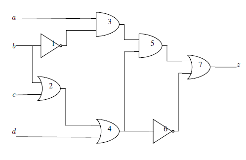
Circuit with 7 logic gates, 4 inputs (\(a, b, c, d\)), and 1 output (\(z\)). The circuit implements function \(z = \overline{b} (ac + ad + \overline{c}\overline{d})\).

Example Requirements¶

To run the code in this example, the following is required.

The requisite information for problem submission through SAPI, as described in Using a D-Wave System
Ocean tools dwavebinarycsp and dwave-system. For the optional graphics, you will also need Matplotlib.

If you installed dwave-ocean-sdk and ran dwave config create, your installation should meet these requirements.

Formulating the Problem as a CSP¶

This example demonstrates two formulations of constraints from the problem’s logic gates:

Single comprehensive constraint:

import dwavebinarycsp

def logic_circuit(a, b, c, d, z):
    not1 = not b
    or2 = b or c
    and3 = a and not1
    or4 = or2 or d
    and5 = and3 and or4
    not6 = not or4
    or7 = and5 or not6
    return (z == or7)

csp = dwavebinarycsp.ConstraintSatisfactionProblem(dwavebinarycsp.BINARY)
csp.add_constraint(logic_circuit, ['a', 'b', 'c', 'd', 'z'])

Multiple small constraints:

import dwavebinarycsp
import dwavebinarycsp.factories.constraint.gates as gates
import operator

csp = dwavebinarycsp.ConstraintSatisfactionProblem(dwavebinarycsp.BINARY)
csp.add_constraint(operator.ne, ['b', 'not1'])  # add NOT 1 gate
csp.add_constraint(gates.or_gate(['b', 'c', 'or2']))  # add OR 2 gate
csp.add_constraint(gates.and_gate(['a', 'not1', 'and3']))  # add AND 3 gate
csp.add_constraint(gates.or_gate(['d', 'or2', 'or4']))  # add OR 4 gate
csp.add_constraint(gates.and_gate(['and3', 'or4', 'and5']))  # add AND 5 gate
csp.add_constraint(operator.ne, ['or4', 'not6'])  # add NOT 6 gate
csp.add_constraint(gates.or_gate(['and5', 'not6', 'z']))  # add OR 7 gate

Note

dwavebinarycsp works best for constraints of up to 4 variables; it may not function as expected for constraints of over 8 variables.

The next line of code converts the constraints into a BQM that we solve by sampling.

# Convert the binary constraint satisfaction problem to a binary quadratic model
bqm = dwavebinarycsp.stitch(csp)

The first approach, which consolidates the circuit as a single constraint, yields a binary quadratic model with 7 variables: 4 inputs, 1, output, and 2 ancillary variables. The second approach, which creates a constraint satisfaction problem from multiple small constraints, yields a binary quadratic model with 11 variables: 4 inputs, 1 output, and 6 intermediate outputs of the logic gates.

You can see the binary quadratic models here: Multiple-Gate Circuit: Further Details.

Minor-Embedding and Sampling¶

Algorithmic minor-embedding is heuristic—solution results vary significantly based on the minor-embedding found.

The next code sets up a D-Wave system as the sampler.

Note

In the code below, replace sampler parameters as needed. If you configured a default solver, as described in Using a D-Wave System, you should be able to set the sampler without parameters as sampler = EmbeddingComposite(DWaveSampler()). You can see this information by running dwave config inspect in your terminal.

from dwave.system.samplers import DWaveSampler
from dwave.system.composites import EmbeddingComposite

# Set up a D-Wave system as the sampler
sampler = EmbeddingComposite(DWaveSampler(endpoint='https://URL_to_my_D-Wave_system/', token='ABC-123456789012345678901234567890', solver='My_D-Wave_Solver'))

Next, we ask for 1000 samples and separate those that satisfy the CSP from those that fail to do so.

response = sampler.sample(bqm, num_reads=1000)

# Check how many solutions meet the constraints (are valid)
valid, invalid, data = 0, 0, []
for datum in response.data(['sample', 'energy', 'num_occurrences']):
    if (csp.check(datum.sample)):
        valid = valid+datum.num_occurrences
        for i in range(datum.num_occurrences):
            data.append((datum.sample, datum.energy, '1'))
    else:
        invalid = invalid+datum.num_occurrences
        for i in range(datum.num_occurrences):
            data.append((datum.sample, datum.energy, '0'))
print(valid, invalid)

For the single constraint approach, 4 runs with their different minor-embeddings yield significantly varied results, as shown in the following table:

Single Constraint¶
Embedding	(valid, invalid)
1	(39, 961)
2	(1000, 0)
3	(998, 2)
4	(316, 684)

You can see the minor-embeddings found here: Multiple-Gate Circuit: Further Details; below those embeddings are visualized graphically.

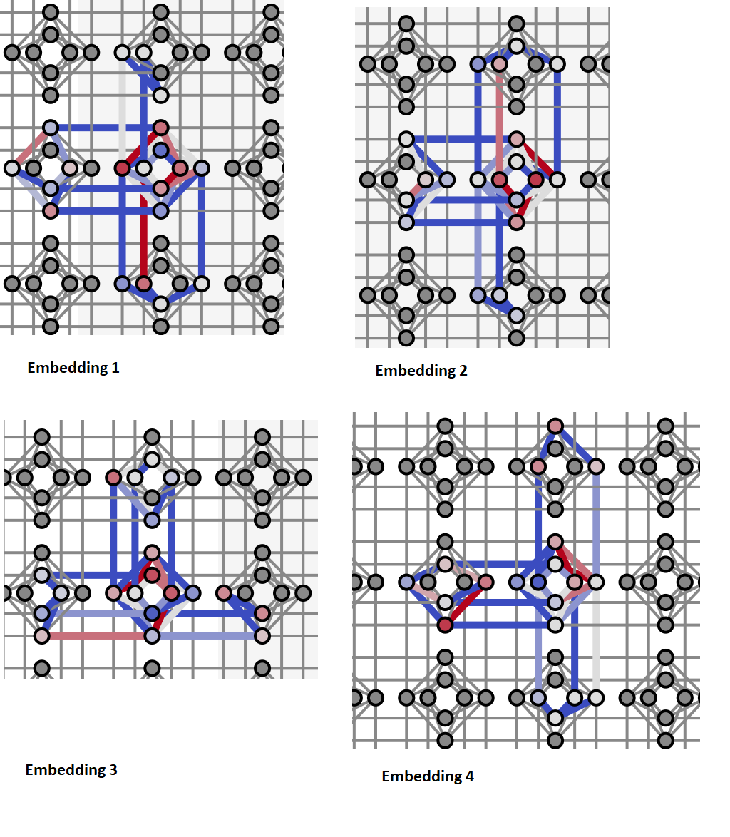
Each of the figure’s 4 panels shows a minor-embedding found for one run of the example code above. The panels show part of the Chimera graph representation of a D-Wave QPU, where each unit cell is rendered as a cross of 4 horizontal and 4 vertical dots representing qubits and lines representing couplers between qubit pairs. Color indicates the strengths of linear (qubit) and quadratic (coupler) biases: darker blue for increasingly negative values and darker red for increasingly positive values.

For the second approach, which creates a constraint satisfaction problem based on multiple small constraints, a larger number of variables (11 versus 7) need to be minor-embedded, resulting in worse performance. However, performance can be greatly improved in this case by increasing the chain strength (to 2 instead of the default of 1).

Multiple Constraints¶
Embedding	Chain Strength	(valid, invalid)
1	1	(7, 993)
2	1	(417, 583)
3	2	(941, 59)
4	2	(923, 77)

You can see the minor-embeddings used here: Multiple-Gate Circuit: Further Details; below those embeddings are visualized graphically.

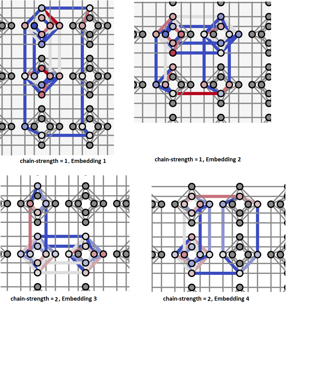
Each of the figure’s 4 panels shows a minor-embedding found for one run of the example code above, as described for the previous figure. Here, the top two panels are for runs with the default chain-strength of 1 and the bottom two for chain-strengths of 2.

Looking at the Results¶

You can verify the solution to the circuit problem by checking an arbitrary valid or invalid sample:

>>> print(next(response.samples()))      
{'a': 1, 'c': 0, 'b': 0, 'not1': 1, 'd': 1, 'or4': 1, 'or2': 0, 'not6': 0,
'and5': 1, 'z': 1, 'and3': 1}

For the lowest-energy sample of the last run, found above, the inputs are \(a, b, c, d = 1, 0, 0, 1\) and the output is \(z=1\), which indeed matches the analytical solution for the circuit,

\[ \begin{align}\begin{aligned}z &= \overline{b} (ac + ad + \overline{c}\overline{d})\\ &= 1(0+1+0)\\ &= 1\end{aligned}\end{align} \]

You can also plot the energies for valid and invalid samples. The example code above converted the constraint satisfaction problem to a binary quadratic model using the default minimum energy gap of 2. Therefore, each constraint violated by the solution increases the energy level of the binary quadratic model by at least 2 relative to ground energy.

>>> import matplotlib.pyplot as plt
>>> plt.ion()
>>> plt.scatter(range(len(data)), [x[1] for x in data], c=['y' if (x[2] == '1')
...             else 'r' for x in data],marker='.')
>>> plt.xlabel('Sample')
>>> plt.ylabel('Energy')

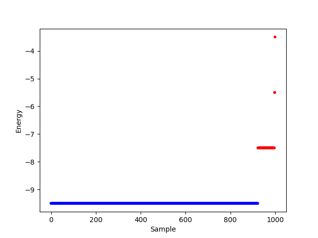
Energies per sample for a 1000-sample problem submission of the logic circuit. Blue points represent valid solutions (solutions that solve the constraint satisfaction problem) and red points the invalid solutions.

You can see in the graph that valid solutions have energy -9.5 and invalid solutions energies of -7.5, -5.5, and -3.5.

>>> for datum in response.data(['sample', 'energy', 'num_occurrences', 'chain_break_fraction']):  
...    print(datum)
...
Sample(sample={'a': 1, 'c': 0, 'b': 1, 'not1': 0, 'd': 1, 'or4': 1, 'or2': 1, 'not6': 0, 'and5': 0, 'z': 0, 'and3': 0}, energy=-9.5, num_occurrences=13, chain_break_fraction=0.0)
Sample(sample={'a': 1, 'c': 1, 'b': 1, 'not1': 0, 'd': 0, 'or4': 1, 'or2': 1, 'not6': 0, 'and5': 0, 'z': 0, 'and3': 0}, energy=-9.5, num_occurrences=14, chain_break_fraction=0.0)
# Snipped this section for brevity
Sample(sample={'a': 1, 'c': 0, 'b': 0, 'not1': 1, 'd': 1, 'or4': 1, 'or2': 0, 'not6': 1, 'and5': 1, 'z': 1, 'and3': 1}, energy=-7.5, num_occurrences=3, chain_break_fraction=0.09090909090909091)
Sample(sample={'a': 1, 'c': 1, 'b': 0, 'not1': 1, 'd': 1, 'or4': 1, 'or2': 1, 'not6': 1, 'and5': 1, 'z': 1, 'and3': 1}, energy=-7.5, num_occurrences=1, chain_break_fraction=0.18181818181818182)
Sample(sample={'a': 1, 'c': 1, 'b': 1, 'not1': 1, 'd': 0, 'or4': 1, 'or2': 1, 'not6': 1, 'and5': 1, 'z': 1, 'and3': 1}, energy=-5.5, num_occurrences=4, chain_break_fraction=0.18181818181818182)
# Snipped this section for brevity
Sample(sample={'a': 1, 'c': 1, 'b': 1, 'not1': 1, 'd': 0, 'or4': 1, 'or2': 1, 'not6': 1, 'and5': 0, 'z': 1, 'and3': 1}, energy=-3.5, num_occurrences=1, chain_break_fraction=0.2727272727272727)

You can see, for example, that sample

Sample(sample={'a': 1, 'c': 1, 'b': 0, 'not1': 1, 'd': 1, 'or4': 1, 'or2': 1, 'not6': 1, 'and5': 1, 'z': 1, 'and3': 1}, energy=-7.5, num_occurrences=1, chain_break_fraction=0.18181818181818182)

has a higher energy by 2 than the ground energy. It is expected that this solution violates a single constraint, and you can see that it violates constraint

Constraint.from_configurations(frozenset([(1, 0, 0), (0, 1, 0), (0, 0, 0), (1, 1, 1)]), ('a', 'not1', 'and3'), Vartype.BINARY, name='AND')

on AND gate 3.

Note also that for samples with higher energy there tends to be an increasing fraction of broken chains: zero for the valid solutions but rising to almost 30% for solutions that have three broken constraints.