Solving Problems on a D-Wave System

This section explains some of the basics of how you can use D-Wave quantum computers to solve problems and how Ocean tools can help.

How a D-Wave System Solves Problems

For quantum computing, as for classical, solving a problem requires that it be formulated in a way the computer and its software understand.

For example, if you want your laptop to calculate the area of a $1 coin, you might express the problem as an equation, \(A=\pi r^2\), that you program as math.pi*13.245**2 in your Python CLI. For a laptop with Python software, this formulation—a particular string of alphanumeric symbols—causes the manipulation of bits in a CPU and memory chips that produces the correct result.

The D-Wave system uses a quantum processing unit (QPU) to solve a binary quadratic model (BQM)[1]: given \(N\) variables \(x_1,...,x_N\), where each variable \(x_i\) can have binary values \(0\) or \(1\), the system finds assignments of values that minimize

\[\sum_i^N q_ix_i + \sum_{i<j}^N q_{i,j}x_i x_j\]

where \(q_i\) and \(q_{i,j}\) are configurable (linear and quadratic) coefficients. To formulate a problem for the D-Wave system is to program \(q_i\) and \(q_{i,j}\) so that assignments of \(x_1,...,x_N\) also represent solutions to the problem.

[1]	The “native” forms of BQM programmed into a D-Wave system are the Ising model traditionally used in statistical mechanics and its computer-science equivalent, shown here, the QUBO.

Ocean software can abstract away much of the mathematics and programming for some types of problems. At its heart is a binary quadratic model (BQM) class that together with other Ocean tools helps formulate various optimization problems. It also provides an API to binary quadratic samplers (the component used to minimize a BQM and therefore solve the original problem), such as the D-Wave system and classical algorithms you can run on your computer.

The following sections describe this problem-solving procedure in two steps (plus a third that may benefit some problems); see the Getting Started examples and system documentation for further description.

1. Formulate the Problem as a BQM.
2. Solve the BQM with a Sampler.
3. Improve the Solutions, if needed, using advanced features.

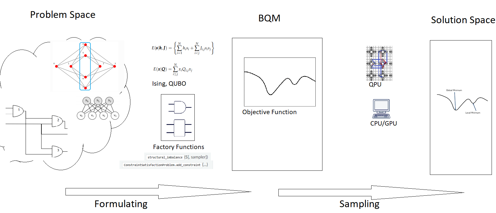
Solution steps: (1) a problem known in “problem space” (a circuit of Boolean gates, a graph, a network, etc) is formulated as a BQM, mathematically or using Ocean functionality and (2) the BQM is sampled for solutions.

Formulate the Problem as a BQM

There are different ways of mapping between a problem—chains of amino acids forming 3D structures of folded proteins, traffic in the streets of Beijing, circuits of binary gates—and a BQM to be solved (by sampling) with a D-Wave system or locally on your CPU/GPU.

For example, consider the problem of determining outputs of a Boolean logic circuit. In its original context (in “problem space”), the circuit might be described with input and output voltages, equations of its component resistors, transistors, etc, an equation of logic symbols, multiple or an aggregated truth table, and so on. You can choose to use Ocean software to formulate BQMs for binary gates directly in your code or mathematically formulate a BQM, and both can be done in different ways too; for example, a BQM for each gate or one BQM for all the circuit’s gates.

The following are two example formulations.

1. The Boolean NOT Gate example, takes a NOT gate represented symbolically as \(x_2 \Leftrightarrow \neg x_1\) and formulates it mathematically as the following BQM:

   \[-x_1 -x_2 + 2x_1x_2\]

   The table below shows that this BQM has lower values for valid states of the NOT gate (e.g., \(x_1=0, x_2=1\)) and higher for invalid states (e.g., \(x_1=0, x_2=0\)).

   Boolean NOT Operation Formulated as a BQM.

   \(x_1\)	\(x_2\)	Valid?	BQM Value
   \(0\)	\(1\)	Yes	\(0\)
   \(1\)	\(0\)	Yes	\(0\)
   \(0\)	\(0\)	No	\(1\)
   \(1\)	\(1\)	No	\(1\)

2. Ocean’s dwavebinarycsp tool enables the following formulation of an AND gate as a BQM:

   >>> import dwavebinarycsp
   >>> import dwavebinarycsp.factories.constraint.gates as gates
   >>> csp = dwavebinarycsp.ConstraintSatisfactionProblem(dwavebinarycsp.BINARY)
   >>> csp.add_constraint(gates.and_gate(['x1', 'x2', 'y1']))  # add an AND gate
   >>> bqm = dwavebinarycsp.stitch(csp)
   

Once you have a BQM that represents your problem, you sample it for solutions.

Solve the BQM with a Sampler

To solve your problem, now represented as a binary quadratic model, you submit it to a classical or quantum sampler. If you use a classical solver running locally on your CPU, a single sample might provide the optimal solution. When you use a probabilistic sampler like the D-Wave system, you typically program for multiple reads.

Note

To configure access to a D-Wave system, see the Using a D-Wave System section.

For example, the BQM of the AND gate created above may look like this:

>>> bqm     
BinaryQuadraticModel({'x1': 0.0, 'x2': 0.0, 'y1': 6.0}, {('x2', 'x1'): 2.0, ('y1', 'x1'): -4.0, ('y1', 'x2'): -4.0}, -1.5, Vartype.BINARY)

The members of the two dicts are linear and quadratic coefficients, respectively, the third term is a constant offset associated with the model, and the fourth shows the variable types in this model are binary.

Ocean’s dimod tool provides a reference solver that calculates the values of a BQM (its “energy”) for all possible assignments of variables. Such a sampler can solve a small three-variable problem like the AND gate created above.

>>> from dimod.reference.samplers import ExactSolver
>>> sampler = ExactSolver()
>>> response = sampler.sample(bqm)    
>>> for datum in response.data(['sample', 'energy']):     
...    print(datum.sample, datum.energy)
...
{'x1': 0, 'x2': 0, 'y1': 0} -1.5
{'x1': 1, 'x2': 0, 'y1': 0} -1.5
{'x1': 0, 'x2': 1, 'y1': 0} -1.5
{'x1': 1, 'x2': 1, 'y1': 1} -1.5
{'x1': 1, 'x2': 1, 'y1': 0} 0.5
{'x1': 0, 'x2': 1, 'y1': 1} 0.5
{'x1': 1, 'x2': 0, 'y1': 1} 0.5
{'x1': 0, 'x2': 0, 'y1': 1} 4.5

Note that the first four samples are the valid states of the AND gate and have lower values than the second four, which represent invalid states.

Ocean’s dwave-system tool enables you to use a D-Wave system as a sampler. In addition to DWaveSampler(), the tool provides a EmbeddingComposite() composite that maps unstructured problems to the graph structure of the selected sampler, a process known as minor-embedding. In our case, the problem is defined on alphanumeric variables \(x1, x2, y1\), that must be mapped to the QPU’s numerically indexed qubits.

Because of the sampler’s probabilistic nature, you typically request multiple samples for a problem; this example sets num_reads to 1000.

>>> from dwave.system.samplers import DWaveSampler
>>> from dwave.system.composites import EmbeddingComposite
>>> sampler = EmbeddingComposite(DWaveSampler())
>>> response = sampler.sample(bqm, num_reads=1000)   
>>> for datum in response.data(['sample', 'energy', 'num_occurrences']):     
...    print(datum.sample, datum.energy, "Occurrences: ", datum.num_occurrences)
...
{'x1': 0, 'x2': 1, 'y1': 0} -1.5 Occurrences:  92
{'x1': 1, 'x2': 1, 'y1': 1} -1.5 Occurrences:  256
{'x1': 0, 'x2': 0, 'y1': 0} -1.5 Occurrences:  264
{'x1': 1, 'x2': 0, 'y1': 0} -1.5 Occurrences:  173
{'x1': 1, 'x2': 0, 'y1': 1} 0.5 Occurrences:  215

Note that the first four samples are the valid states of the AND gate and have lower values than invalid state \(x1=1, x2=0, y1=1\).

Improve the Solutions

More complex problems than the ones shown above can benefit from some of the D-Wave system’s advanced features and Ocean software’s advanced tools.

The mapping from problem variables to qubits, minor-embedding, can significantly affect performance. Ocean tools perform this mapping heuristically so simply rerunning a problem might improve results. Advanced users may customize the mapping by directly using the minorminer tool or setting a minor-embedding themselves (or some combination).

D-Wave systems offer features such as spin-reversal (gauge) transforms and anneal offsets, which reduce the impact of possible analog and systematic errors.

You can see the parameters and properties a sampler supports. For example, Ocean’s dwave-system lets you use the D-Wave’s virtual graphs feature to simplify minor-embedding. The following example maps a problem’s variables x, y to qubits 1, 5 and variable z to two qubits 0 and 4, and checks some features supported on the D-Wave system used as a sampler.

Attention

D-Wave’s virtual graphs feature can require many seconds of D-Wave system time to calibrate qubits to compensate for the effects of biases. If your account has limited D-Wave system access, consider using FixedEmbeddingComposite() instead.

>>> from dwave.system.samplers import DWaveSampler
>>> from dwave.system.composites import VirtualGraphComposite
>>> DWaveSampler().properties['extended_j_range']
[-2.0, 1.0]
>>> embedding = {'x': {1}, 'y': {5}, 'z': {0, 4}}
>>> sampler = VirtualGraphComposite(DWaveSampler(), embedding)
>>> sampler.parameters
{u'anneal_offsets': ['parameters'],
 u'anneal_schedule': ['parameters'],
 u'annealing_time': ['parameters'],
 u'answer_mode': ['parameters'],
 'apply_flux_bias_offsets': [],
 u'auto_scale': ['parameters'],
>>>  # Snipped above response for brevity

Note that the composed sampler (VirtualGraphComposite() in the last example) inherits properties from the child sampler (DWaveSampler() in that example).

See the resources under Additional Tutorials and the System Documentation for more information.